
Assumptions
An assumption is an uncertain input cell with a probability distribution. In each simulation trial, OpenRiskSim replaces the cell's value with a number drawn from that distribution and recalculates the workbook.
Defining an assumption
- Select the cell holding the input value (e.g. the price
26), not its label. - Click Simulation → Define assumption, Alt+A, or right-click → Define assumption.
- Pick the distribution in the gallery, adjust the parameters and click OK.
The cell turns green and appears in the Model explorer.
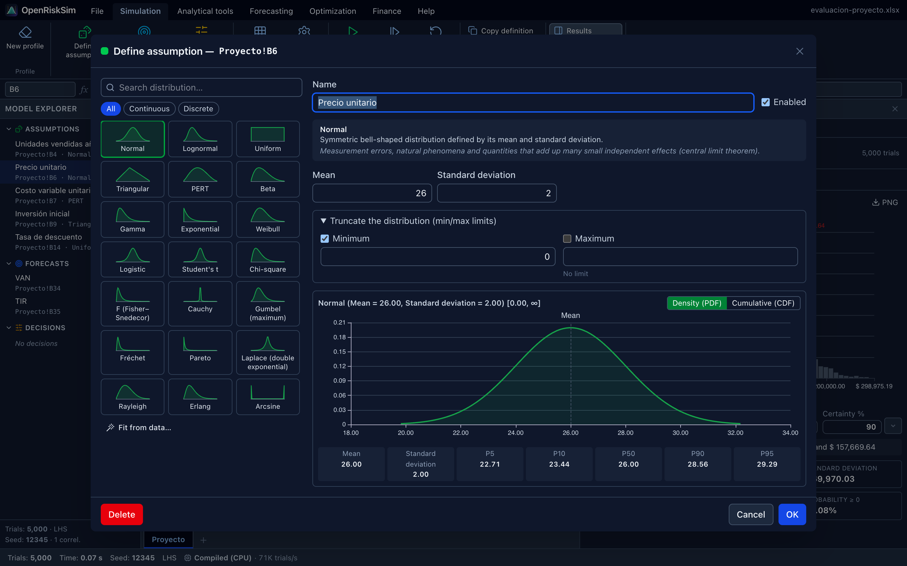
Parts of the dialog
| Part | Purpose |
|---|---|
| Search distribution… and the All / Continuous / Discrete filters | Quickly find one of the 33 distributions. Each card shows the typical shape. |
| Name | Proposed automatically from the nearest text to the left (or above) the cell, e.g. “Unit price”. You can change it. |
| Enabled | If unticked, the assumption is kept but not simulated: the cell keeps its fixed value. Useful to compare “with and without” a variable's uncertainty. |
| Description box | What the distribution is and its typical use. |
| Parameters | Fields specific to each distribution (Mean, Standard deviation, Minimum, Most likely, Maximum…). Invalid values are flagged in red. |
| Truncate the distribution (min/max limits) | Restricts the possible values (see below). |
| Density (PDF) / Cumulative (CDF) chart | Preview of the chosen distribution with the mean marked, and the Mean, Standard deviation, P5, P10, P50, P90 and P95. |
| Fit from data… | Chooses the distribution that best describes your historical data (see below). |
| Delete | Removes the assumption (only if the cell already had one). |
Suggested values
When you pick a distribution, its parameters are proposed around the cell's current value (e.g. for a price of 26, a Triangular from 23.4 to 28.6 with mode 26). They are just a starting point: replace them with your own estimates.
Common warnings
- “The cell contains a formula…”: during the simulation the formula is replaced by random values (restored afterwards). Assumptions are normally defined on cells with constant values; if the cell is a formula, you probably want the assumption on one of the cells it depends on.
- “The cell does not contain a number…”: you are on a label or an empty cell. Move to the value cell.
Truncation
Open Truncate the distribution, tick Minimum and/or Maximum and type the limit. Values outside the range are never generated; probability is redistributed inside it (technically the inverse CDF is applied on the restricted interval).
Typical uses:
- A Normal for units sold or price with minimum 0, so they never go negative (as in the “Project evaluation” example).
- A Normal interest rate limited to a realistic range (e.g. 2%–16%).
WARNING
Truncation changes the distribution's mean and standard deviation. If you truncate heavily (e.g. cut a Normal at its mean), the resulting mean shifts. Check the preview: the P5–P95 values and the mean already include truncation.
Custom distribution (your own data)
The Custom distribution is defined by a list of Values (separated by spaces, ; or line breaks) and, optionally, their Probabilities:
- With probabilities → discrete distribution. Scenario example: values
80; 100; 130with probabilities0.25; 0.5; 0.25. If they don't add up to 1, they are normalised. - Without probabilities → continuous empirical distribution that resamples your data, interpolating between points. Useful when you have historical data that doesn't look like any standard distribution.
With Load values from a range you can pull the values straight from the sheet (type the range, e.g. Data!B2:B37, or use the current selection) and click Load.
Fit from data
If you have historical data (last 36 months of prices, weekly demand…):
- In the dialog click Fit from data…
- Enter the range with the data (at least 5 numeric values) and click Fit.
- You'll see the 8 best distributions ranked by AIC (lower is better), with their estimated parameters. Click Use on the one you prefer: its parameters are copied into the assumption.
For a fuller analysis (Kolmogorov–Smirnov, Anderson–Darling and χ² tests, P–P and Q–Q plots) use Analytical tools → Distribution fitting, which can also create the assumption directly.
Copying and pasting definitions
To use the same distribution in many cells (e.g. each year's growth):
- Select the cell that already has the assumption and click Simulation → Copy definition.
- Select the target range (may be many cells) and click Paste definition.
Each cell gets an independent copy of the definition, named after its own label. Existing assumptions are replaced. Delete definition removes every definition (assumptions, forecasts or decisions) in the selected range. Copy/paste also works for forecasts and decision variables.
Copying cells doesn't copy definitions
Ctrl+C / Ctrl+V copy values and formulas, as in Excel. Model definitions are only copied with Copy definition / Paste definition.
Editing or deleting
- Click Define assumption again on the cell (or the edit icon in the Model explorer).
- To delete: the dialog's Delete button, the bin icon in the explorer, or Delete definition.
- New profile deletes the whole model at once (the sheet doesn't change).
Choosing a distribution
There is no universally “right” distribution: choose the one that best represents what you know about the variable, and justify it in your report.
| If you have… | Use… | Why |
|---|---|---|
| A minimum, a most likely value and a maximum (expert opinion, quotes) | Triangular or PERT | Three easy-to-get estimates. PERT gives more weight to the most likely value and has softer tails; Triangular is more conservative (more spread). |
| Only a range, no preferred value | Uniform | All values in the range equally likely. Represents maximum ignorance within the range. |
| A mean and a symmetric spread (errors, sums of many effects) | Normal (truncated if it can't be negative) | Classic, symmetric. |
| A positive, right-skewed variable (prices, costs, incomes, property values) | Lognormal | Never negative; grows multiplicatively. Its parameters are the mean and sd of the variable, not of its log. |
| Enough historical data (ideally ≥ 30) | Distribution fitting or Custom | Let the data decide. |
| Counts of events in a period (customers per hour, failures per month) | Poisson | Independent events at a constant rate λ. |
| An event that happens or not (permit approved, tender won) | Bernoulli (yes/no) | 1 with probability p, 0 otherwise. Multiply the event's effect by the cell. |
| Number of successes in n tries (distributors signing out of 20 contacted) | Binomial | n independent trials with probability p. |
| Bounded proportions or percentages (market share, occupancy rate) | Beta | Very flexible on an interval [min, max]. |
| Times between events, durations | Exponential, Gamma, Weibull, Erlang | Positive and skewed; Weibull is standard in reliability. |
| Extreme values (largest flood, worst loss) | Gumbel, Fréchet, Pareto | Heavy tails. |
| Discrete scenarios with subjective probabilities (pessimistic / base / optimistic) | Custom with probabilities | Exactly your scenarios. |
| A constant you want to “switch off” without deleting the assumption | Fixed value (or untick Enabled) | Removes the uncertainty temporarily. |
A rule of thumb for coursework
For most project variables (price, quantity, unit cost, investment) a Triangular or PERT with pessimistic / most likely / optimistic estimates is enough and easy to justify. Use a Normal when a source gives you a mean and a standard deviation, and fitting when you have historical series. The sensitivity tools tell you which variables deserve more effort.
See the distribution reference for the parameters of all 33 distributions.
Which cells should be assumptions?
- Model inputs with relevant uncertainty: price, volume, unit costs, investment, growth rate, discount rate (if not fixed by policy).
- Not calculated cells (revenue = price × quantity): they change on their own.
- Not variables with no influence: if the tornado shows a variable barely moves the NPV, keep it fixed and simplify the model.
- If a variable repeats every year (e.g. each year's price), you can put one assumption on the year-1 price and project the rest with a growth formula, or one assumption per year. The former models a permanent shock; the latter, independent yearly variations (which tend to cancel out). Choose according to your project, or use correlations between years.