
Interpreting results
When the simulation finishes, the Results panel shows one tab per forecast (e.g. VAN and TIR — NPV and IRR — in the example) and an Overlay tab. Each forecast has three inner tabs: Histogram, Statistics and Percentiles.
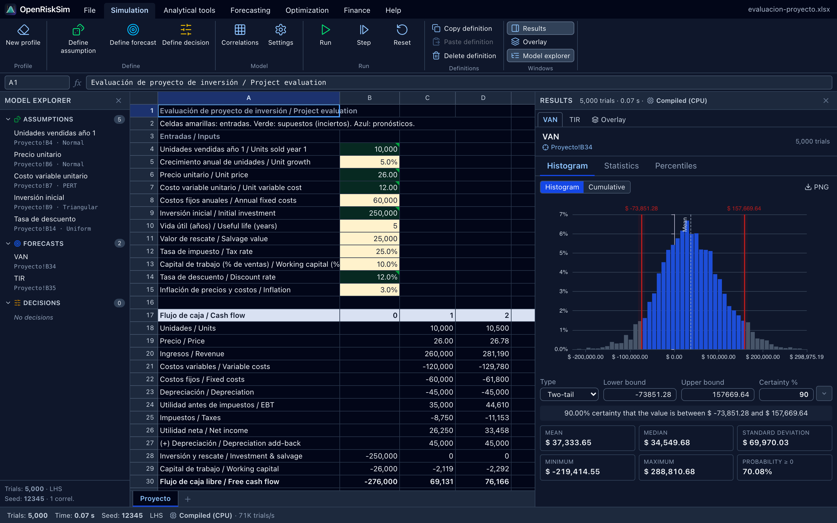
The header shows the forecast's name, its cell (click to go there) and the number of valid trials; if some trials failed, it says how many and what share.
Histogram and cumulative distribution
The Histogram / Cumulative switch changes the view:
- Histogram: each bar shows the percentage of trials that fell in that interval. The dashed line marks the mean. It shows the shape of the risk: where results concentrate, whether it is symmetric or has a long tail.
- Cumulative: for each value x, the probability of a result less than or equal to x. The most direct way to read probabilities: find NPV = 0 on the horizontal axis and read the probability of loss on the vertical one.
The PNG button downloads the chart as an image for your report.
Certainty
Certainty is the probability that the forecast falls in an interval. It is controlled by four fields under the chart:
| Field | Use |
|---|---|
| Type | Two-tail (between two bounds), Left-tail ≤ (at most an upper bound) or Right-tail ≥ (at least a lower bound). |
| Lower bound / Upper bound | Type a value and the certainty is recomputed. |
| Certainty % | Type a percentage and the bounds are recomputed. The small ▾ drop-down to its right (Quick certainties (80 / 90 / 95 / 99%)) applies one of those levels in one click. |
You can also drag the red lines on the histogram. Bars inside the interval are blue; those outside, grey. A sentence summarises the result, e.g. “90.00% certainty that the value is between $ −73,851.28 and $ 157,669.64”.
When a forecast opens, certainty starts at Two-tail with the Initial chart certainty set in the forecast: 90% by default (the interval leaving 5% of trials on each side). If you change that value by editing the forecast, the band updates at once (keeping the tail type), without re-running.
The most common questions
| Question | How to answer it |
|---|---|
| Probability that the project is profitable? | Right-tail ≥, Lower bound 0 → Certainty % = P(NPV ≥ 0). |
| Probability of loss? | Left-tail ≤, Upper bound 0 → Certainty % = P(NPV ≤ 0). (Or 100% minus the previous one.) |
| Between which values will the NPV fall with 90% confidence? | Two-tail, Certainty % 90 → read the bounds. |
| Probability that the IRR beats a 12% hurdle rate? | In the IRR window: Right-tail ≥, Lower bound 0.12 (bounds are typed as fractions even when the forecast is shown as %). |
| NPV exceeded with 95% probability? | Right-tail ≥, Certainty % 95 → the lower bound is that value (the 5th percentile). |
The certainty ranges you set are also used in the charts of the exported report.
Quick statistics
Under the chart there are six cards: Mean, Median, Standard deviation, Minimum, Maximum and Probability ≥ 0. The last one immediately answers the profitability question when the forecast is an NPV.
Statistics tab
| Statistic | Meaning | How to use it |
|---|---|---|
| Valid trials | Number of trials without errors. | If much lower than the configured trials, check the errors. |
| Mean | Average of all results: the expected value. | The project's expected NPV — the headline figure of the risk analysis. |
| Median | Value with half the trials below and half above (50th percentile). | If very different from the mean, the distribution is skewed. |
| Mode | Most frequent value (for continuous results, the centre of the tallest bar). | Indicative. |
| Standard deviation | Typical spread around the mean, in the same units (sample estimator, n − 1). | Classic measure of absolute risk: the larger, the more uncertain. |
| Variance | Standard deviation squared. | Used in formulas; less intuitive. |
| Coefficient of variation | Standard deviation / |mean|. | Relative risk: compares projects of different sizes. CV above 1 (100%) means the spread exceeds the expected value. |
| Minimum / Maximum / Range | Worst and best simulated result and their difference. | Depend heavily on the number of trials; prefer percentiles (P5, P95). |
| Skewness | 0 = symmetric; > 0 = long tail towards high values; < 0 = long tail towards low values. | Negative skew in an NPV means unlikely but possible large losses. |
| Kurtosis (excess) | 0 = Normal-like tails; > 0 = heavy tails (more extreme values); < 0 = light tails. | High kurtosis warns of extreme events. |
| Standard error of the mean | Standard deviation / √n: how much the mean would vary if you repeated the simulation. | If large relative to the mean, add trials. |
| 95% CI of the mean | Confidence interval for the mean (Student's t), at the forecast's Confidence of the mean interval level: 95% by default; the row is called, e.g., 99% CI of the mean if you choose 99%. | Precision of the expected-value estimate. It is not the range where the NPV will fall (use certainty for that). |
| 10th / 90th percentile | Values with 10% of trials below / above. | “Reasonable” pessimistic and optimistic cases. |
| Probability ≥ 0 | Share of trials with a result ≥ 0. | P(NPV ≥ 0). |
| Trials with errors | Trials where the forecast couldn't be computed. | Ideally 0. |
Statistics follow Excel's conventions (STDEV.S, SKEW, KURT, PERCENTILE.INC), so you can verify them by exporting the simulation data to .xlsx.
Three intervals not to confuse
OpenRiskSim shows three kinds of interval with similar-looking “levels” (90%, 95%…), but they answer different questions:
| Interval | Where it appears | Question it answers | What happens with more trials |
|---|---|---|---|
| Certainty band of the simulated distribution | Forecast histogram (Certainty %) | Between which values will the outcome (this project's NPV) fall with 90% probability? | It stabilises but does not shrink: it reflects the project's real uncertainty. |
| Confidence interval of the mean | Statistics tab (95% CI of the mean) | How precise is the simulation's estimate of the expected value? | It shrinks (≈ 1/√n): with enough trials the mean is known very precisely. |
| Prediction interval of a time-series forecast | Forecasting → Time series (95% interval) | Between which values will the series' next observation be (sales in month 13)? | Depends on the historical data, not on trials; it widens with the horizon. |
Example with the “Project evaluation” model (10,000 trials): the 90% certainty band of the NPV goes from about −$74,000 to $157,000, while the 95% CI of the mean is roughly $37,387 ± $1,400. Saying “the NPV will be between $36,000 and $39,000 with 95% confidence” would be a serious mistake: that is the precision of the mean, not the range of the NPV.
Regression
The confidence intervals of the coefficients of a regression are of the second kind: they show how precisely each coefficient was estimated, not the range of Y.
Percentiles tab
Table with the 1st, 5th, 10th, 15th, …, 90th, 95th and 99th percentiles. The p-th percentile is the value below which p% of the trials fall. For example, if the NPV's 5th percentile is −$74,000, there is a 5% probability that the NPV is even worse.
Project VaR
The 5th (or 1st) percentile of the NPV is a Value at Risk-type measure: “with 95% confidence, the project won't lose more than X”.
Overlay chart
The Overlay tab (or Simulation → Overlay) draws several forecasts on the same chart, as density or cumulative. Use it to compare alternatives: e.g. the project NPV with and without financing, or two plant sizes. A curve shifted to the right has higher values; a wider one, more risk. For more options (number of bins, summary) use Analytical tools → Overlay chart.
Compare on the same scale
Overlays make sense between forecasts of the same kind (two NPVs, two profits). Don't overlay an NPV with an IRR.
Sensitivity
To learn which assumptions drive the forecast's risk use Analytical tools → Sensitivity (uses the last simulation) and Tornado.
Writing the interpretation in a report
A good risk-analysis paragraph states: what was simulated (assumptions and distributions, correlations), how (trials, method, seed), the expected value, the spread, the probability of loss, a certainty interval and the most influential variables. Example with the “Project evaluation” model (10,000 trials):
A Monte Carlo simulation of 10,000 trials (Latin hypercube sampling, seed 12345) was run on the project's cash flow, modelling as uncertain the year-1 units sold (Normal, μ = 10,000, σ = 1,500), the unit price (Normal, μ = $26, σ = $2), the unit variable cost (PERT 10.5 – 12 – 15), the initial investment (Triangular 220,000 – 250,000 – 310,000) and the discount rate (Uniform 10% – 14%), with a −0.5 correlation between price and units.
The expected NPV is $37,387, below the base-case NPV ($58,250), with a standard deviation of $70,370 (CV = 1.88). There is a 30.3% probability of a negative NPV. With 90% certainty the NPV will lie between −$74,287 and $157,001. The expected IRR is 16.2%, with a 69.8% probability of exceeding the 12% reference discount rate.
Sensitivity analysis shows that units sold (33.6% of the NPV variance), price (29.7%) and unit variable cost (24.5%) explain about 88% of the risk; investment and discount rate have a smaller effect. Further market research is recommended to reduce uncertainty about volume and price before committing to the investment.
The tutorial shows how to obtain those figures.