
Forecasting
The Forecasting tab contains three tools to project variables from historical data. Their results help you define better-grounded assumptions: e.g. use the demand forecast as the expected value and its prediction interval to choose the spread.
“Forecast” has two meanings
In this tab, forecast means projecting a series into the future. Don't confuse it with the model's forecast cells (the blue output cells of the simulation), which Risk Simulator also calls forecasts.
Time series
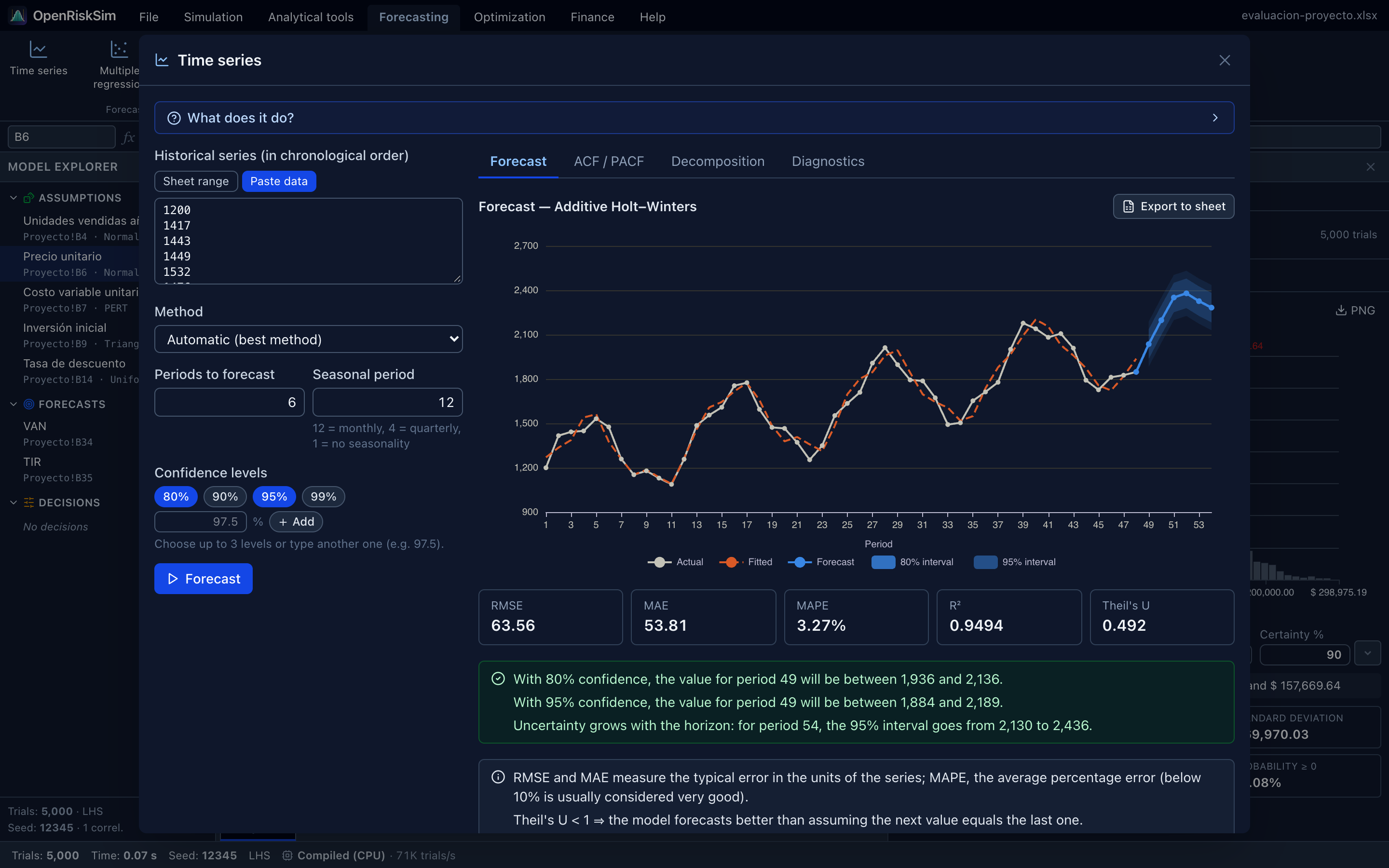
Purpose. Forecasts a series (monthly sales, demand, prices…) several periods ahead, with prediction intervals at the confidence levels you choose (80% and 95% by default).
How to use it.
- Historical series (in chronological order): a sheet range or pasted data. A single column, oldest to newest, without gaps.
- Method (see table).
- Periods to forecast (6 by default) and, for seasonal methods, Seasonal period (12 = monthly, 4 = quarterly, 1 = no seasonality). Depending on the method, Averaging window, the ARIMA (p, d, q) order or the Trend type appear.
- Confidence levels of the prediction intervals (see below).
- Click Forecast.
Confidence levels
The Confidence levels picker shows up to 3 intervals at once:
- The 80%, 90%, 95% and 99% buttons switch each level on or off (80% and 95% by default).
- In Other level (%) you can type any level between 50 and 99.9%, decimals included (e.g.
97.5), and click Add or press Enter. Custom levels appear as buttons with an ✕ to remove them. - At least one level always remains. With three already selected, the message “At most 3 levels: remove one before adding another.” asks you to remove one first.
Changing the levels after forecasting recomputes the intervals at once with the same data and method. The Automatic method uses the same levels for every candidate.
Methods and when to use them
| Method | When to use it |
|---|---|
| Automatic (best method) | When unsure. Tries moving average, simple smoothing, Holt, damped Holt, Holt–Winters (with at least two full cycles), auto-ARIMA and a linear trend; fits them on the first 80% of the data, measures RMSE on the last 20% and keeps the lowest. The Method comparison table shows the ranking. |
| Moving average | Series without trend or seasonality, to smooth noise. Flat forecast. |
| Simple exponential smoothing | No trend or seasonality; weights recent data more (parameter α). |
| Holt (linear trend) | Series with a trend (sustained growth or decline). |
| Damped Holt | A trend expected to flatten over time; usually more prudent in the long run. |
| Additive Holt–Winters (seasonal) | Trend + seasonality of constant size (e.g. +200 units every December). |
| Multiplicative Holt–Winters (seasonal) | Seasonality proportional to the level (e.g. +15% every December). Requires positive data. |
| ARIMA(p, d, q) | When you know the order (from the ACF/PACF plots). d = number of differences to remove the trend. |
| Auto-ARIMA | Chooses d with Dickey–Fuller tests, then tries every p, q ≤ 3 and keeps the lowest AIC (like R's auto.arima). |
| Trend line | Linear, Exponential, Logarithmic, Power, Polynomial (degree 2) or (degree 3), like Excel trendlines. Handy for short series. |
Seasonal methods need at least two full cycles (24 monthly points with period 12).
How to read it
Forecast tab. The chart shows the Actual series, the model's Fitted values and the Forecast with one band per chosen level (80% interval, 95% interval, 97.5% interval…): the higher the level, the wider the band, and the further out, the wider too. Below:
| Metric | Meaning |
|---|---|
| RMSE | Root mean squared error, in the series' units. Penalises large errors more. |
| MAE | Mean absolute error, in the series' units. |
| MAPE | Mean absolute percentage error. Below 10% is usually very good; 10–20% good. Useless if the series has zeros. |
| R² | Share of the series' variation explained by the fitted values. |
| Theil's U | Compares the model with the naive forecast “next value equals the last one”. U < 1 ⇒ better than naive; U ≥ 1 ⇒ adds nothing, try another method. |
A box spells out the interpretation of each level for the first forecast period, e.g. “With 95% confidence, the value for period 25 will be between 1,180 and 1,420.”, and reminds you that “Uncertainty grows with the horizon”, giving the highest level's interval for the last period.
You also get the Estimated parameters (α, β, γ, ARIMA coefficients…) and the Forecast values table, with the columns Period, the lower bounds (Low 95%, Low 80%, widest to narrowest), the Forecast and the upper bounds (High 80%, High 95%). Export to sheet creates a sheet with Period, Actual, Fitted, Forecast and a Lower X% / Upper X% column pair for each level.
A prediction interval, not a confidence interval of the mean
These intervals show where each future value of the series will fall, including its own variability: that is why they are wide and widen with the horizon. They are not the precision of the forecast mean. See Three intervals not to confuse.
ACF / PACF tab. Autocorrelation and partial autocorrelation by Lag. Bars beyond the dashed lines (±1.96/√n) are significant. Peaks at lags 12, 24… suggest monthly seasonality; a slowly decaying ACF suggests a trend (non-stationary series). Classic ARIMA guide: a PACF cutting off at lag p suggests AR(p); an ACF cutting off at q suggests MA(q).
Decomposition tab. Splits the Observed series into Trend, Seasonal component (pattern repeating each period) and Residual (irregular).
Diagnostics tab.
- Augmented Dickey–Fuller test: p < 0.05 ⇒ the series is stationary; p ≥ 0.05 ⇒ it has a trend or unit root and ARIMA will need d ≥ 1.
- Ljung–Box test on residuals: p ≥ 0.05 ⇒ residuals are white noise (the model captured the structure); p < 0.05 ⇒ autocorrelation remains and the model can be improved.
- Candidate seasonal periods with their Strength (near 1 ⇒ strong seasonal pattern).
From forecast to assumption
To use the year-1 sales forecast in your simulation: set a Normal assumption with mean = forecast value and standard deviation ≈ (upper 95% − lower 95%) / 3.92 (with the 95% level selected; for 90% divide by 3.29 and for 80% by 2.56). If the band is asymmetric, a Triangular or PERT using the 95% bounds as minimum and maximum is a simple alternative.
Multiple regression
Purpose. Estimates a linear equation Y = b₀ + b₁·X₁ + … + bₖ·Xₖ by least squares: e.g. demand as a function of price, income and advertising. Equivalent to the Regression tool of Excel's Analysis ToolPak.
How to use it.
- Dependent variable (Y): a single column.
- Independent variables (X): one or more ranges (Add X range); each range can have several columns. Tables pasted from Excel are tab-separated.
- First row has headers: Detect automatically, yes or no. Headers name the variables.
- Include constant (b₀) (ticked by default).
- Stepwise regression, optional, with p to enter (0.05) and p to remove (0.10).
- Confidence level of the coefficient confidence intervals: a single level, 95% by default (like Excel). Pick 80, 90, 95 or 99%, or type another between 50 and 99.9% (e.g.
97.5) and click Use. Changing it after estimating re-runs the regression with the same data. - Click Estimate. Rows with missing or non-numeric data are skipped (the count is shown).
How to read it.
| Output | Reading |
|---|---|
| R² / Adjusted R² | Share of Y's variation explained by the model. Adjusted penalises useless variables: use it to compare models with different numbers of X. |
| F statistic and its p-value | p < 0.05 ⇒ the model as a whole is significant. |
| Standard error of regression | Typical prediction error, in Y units. |
| Coefficients | Each is the change in Y per extra unit of that X, holding the others constant. With Standard error, t statistic, p-value and the CI at the chosen level (column 95% CI, 90% CI…; when exported, X% CI lower and X% CI upper). A * marks p < 0.05 (significant). |
| VIF | Variance inflation factor. VIF > 10 (⚠) ⇒ multicollinearity: those X are highly correlated and their coefficients unstable. |
| Durbin–Watson | Near 2 ⇒ no residual autocorrelation. Below 1.5 or above 2.5 ⇒ possible autocorrelation (common with time series): p-values may be unreliable. |
| ANOVA table | Sums of squares for Regression, Residual and Total, with df and mean squares. |
| Residual plots | Residuals vs fitted, Actual vs fitted, Residuals in order and Residual histogram. Residuals should be a patternless cloud around 0. A funnel ⇒ heteroscedasticity; a curve ⇒ a missing non-linear relationship. |
The tool also writes an interpretation of each significant coefficient, e.g. “For each additional unit of ‘Advertising’, ‘Sales’ increases by 3.2 units, all else equal (significant at 5%). With 95% confidence, the coefficient of ‘Advertising’ lies between 2.1 and 4.3.” The coefficient CI shows how precisely the effect was estimated, not the range of Y. Significance (*) is always judged at 5%, regardless of the level chosen for the intervals.
Stepwise regression. At each step adds the most significant variable (if its p-value is below p to enter) and removes those that stop being significant (p-value above p to remove). The result lists the Selected variables. Useful with many candidate X, but no substitute for economic reasoning: a variable without theoretical meaning shouldn't stay just because of its p-value.
Stochastic processes
Purpose. Simulates future paths of a financial variable (commodity price, exchange rate, interest rate) and shows a fan chart of percentiles over time.
How to use it.
- Choose the Process:
- Geometric Brownian motion: the value grows at a Drift (annual growth) with shocks proportional to the Annual volatility. The classic stock-price model; never negative.
- Mean reversion (Ornstein–Uhlenbeck): the variable tends back to a Long-run mean at a given Reversion speed; volatility is in the variable's units. Suitable for interest rates, commodity prices or costs.
- Jump diffusion (Merton): like geometric Brownian motion plus occasional Jumps per year with a Mean jump size and Jump std. dev. (crises, news).
- Set the Initial value, Δt (years per step) (1/12 = monthly, 1/252 = trading day), Steps (36 by default) and Paths (1,000 by default, up to 20,000), and the seed.
- Choose the Confidence levels of the fan bands: up to 3, 50%, 80% and 90% by default (same picker as in Time series; levels such as
97.5are accepted). - Click Simulate.
Estimate parameters from historical data. Paste or select a Historical price series, set the Data Δt (years) and click Estimate: the tool computes drift and volatility (geometric Brownian motion) or long-run mean, speed and volatility (mean reversion), and takes the last data point as the initial value.
How to read it. The chart shows the Median and one band per level with its percentiles: with the default levels, Central 90% (P5–P95), Central 80% (P10–P90) and Central 50% (P25–P75); a 95% level is labelled Central 95% (P2.5–P97.5). Some Sample paths are drawn as well. The bands are percentiles of the simulated paths at each time (a certainty band, like the one on a forecast histogram), and changing the levels recomputes them without re-simulating. The conclusion uses the highest level: “At the end of the horizon (3 years) the median is X and there is a 90% probability that the value lies between A and B”, and the end-of-horizon table lists each band's interval. The Distribution at the end of the horizon histogram can help you define an assumption: e.g. a PERT with the last period's P5, median and P95 as minimum, most likely and maximum. Export to sheet copies, for each time, the percentiles (P5, P10, P25, P50, P75, P90, P95) and the Lower X% / Upper X% bounds of every band.