
Tutorial: risk analysis of an investment project
This tutorial walks end to end through a risk analysis like the ones assigned in project evaluation courses: from the deterministic cash flow to the final recommendation. It uses the “Project evaluation” example model shipped with the app, so you can reproduce exactly the same figures.
Estimated time: 45 minutes. Prerequisite: the quick start.
1. The case
A company is considering launching a product over a 5-year horizon:
| Variable | Base value | Cell |
|---|---|---|
| Units sold in year 1 | 10,000 | B4 |
| Annual unit growth | 5% | B5 |
| Unit price (year 1) | $26.00 | B6 |
| Unit variable cost (year 1) | $12.00 | B7 |
| Annual fixed costs | $60,000 | B8 |
| Initial investment (fixed assets) | $250,000 | B9 |
| Useful life (straight-line depreciation) | 5 years | B10 |
| Salvage value | $25,000 | B11 |
| Tax rate | 25% | B12 |
| Working capital | 10% of next year's sales | B13 |
| Discount rate (hurdle rate) | 12% | B14 |
| Price and cost inflation | 3% | B15 |
2. Build the cash flow
Three options. Pick one:
A. Use the example (recommended for this tutorial). File → Examples → Project evaluation. It already contains the cash flow (rows 17–31) and the indicators (rows 33–38). To start the risk model from scratch, click Simulation → New profile: it deletes assumptions and forecasts but leaves the sheet untouched.
B. Use the Project evaluator. Finance → Project evaluator: fill in the general data, per-year data and (if applicable) financing, and click Export with formulas. A Project sheet is created with the cash flow as live formulas, and a message tells you which cell holds the NPV and where price and units are, ready for assumptions. See Finance → Project evaluator.
C. Open your own Excel file. File → Open your project's .xlsx. Make sure the NPV is a formula depending on the input cells (not a pasted value).
Check that the model is “live”
Before simulating, change an input by hand (e.g. the price from 26 to 20) and check that the NPV changes. If it doesn't, there are pasted values instead of formulas or broken references. Then undo (Ctrl+Z).
3. Deterministic result
With the base values, the example gives:
| Indicator | Cell | Value | Decision |
|---|---|---|---|
| NPV (12%) | B34 | $58,250 | NPV > 0 ⇒ accept |
| IRR | B35 | 19.1% | IRR > 12% ⇒ accept |
| Payback | B36 | 3.51 years | Within the horizon |
| Profitability index | B37 | 1.21 | > 1 |
| EAA | B38 | $16,159 per year | > 0 |
Free cash flow: year 0 −$276,000 (investment + working capital), years 1–5: $69,131, $76,166, $83,843, $92,218 and $164,818 (the last includes salvage and recovery of working capital).
The deterministic conclusion would be “the project is worth it”. The risk-analysis question is: with what probability?
4. Identify the critical variables (tornado)
Not every variable deserves to be an assumption. To find out which matter, run a sensitivity analysis before simulating. OpenRiskSim's tornado needs assumptions already defined, so in practice: provisionally define wide assumptions on all candidate inputs, run the tornado, then refine the critical ones.
With the step-5 assumptions defined, open Analytical tools → Tornado, choose the VAN (NPV) forecast, keep the percentiles at 10 and 90 and click Calculate:
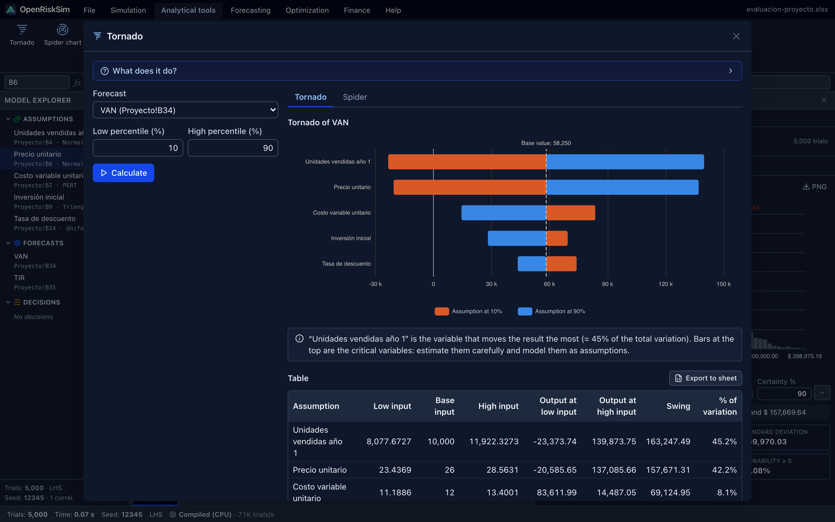
| Assumption | NPV at P10 | NPV at P90 | Swing | % of variation |
|---|---|---|---|---|
| Units sold year 1 | −$23,374 | $139,874 | $163,247 | 45.2% |
| Unit price | −$20,586 | $137,086 | $157,671 | 42.2% |
| Unit variable cost | $83,612 | $14,487 | $69,125 | 8.1% |
| Initial investment | $69,373 | $28,114 | $41,259 | 2.9% |
| Discount rate | $73,998 | $43,560 | $30,438 | 1.6% |
Reading: units and price are by far the critical variables: each one alone, moving between its P10 and P90, flips the sign of the NPV. Variable cost has an intermediate effect; investment and rate, a smaller one. In bars with swapped colours (cost, investment and rate: blue, “assumption at 90%”, on the left) the relationship is inverse: if the variable rises, the NPV falls.
TIP
Fixed costs, tax rate or salvage value were not modelled as uncertain in this example. If they carry relevant uncertainty in your project, include them and check their weight in the tornado.
5. Define the assumptions (with justification)
For each critical variable, define an assumption (Simulation → Define assumption) and write down in your report why you chose that distribution and those parameters. This is how the example does it:
| Assumption | Cell | Distribution | Justification (sample wording) |
|---|---|---|---|
| Units sold year 1 | B4 | Normal (μ = 10,000; σ = 1,500), truncated at minimum 0 | The market study estimates demand of 10,000 units with a ±15% standard error. The normal reflects symmetric errors; truncated at 0 because sales can't be negative. |
| Unit price | B6 | Normal (μ = 26; σ = 2), truncated at minimum 0 | Competitors' average price: $26, with an observed spread of ±$2. |
| Unit variable cost | B7 | PERT (10.5 – 12 – 15) | Supplier quotes: most likely $12; negotiable minimum $10.50 and maximum, if input prices rise, $15 (skewed upwards). |
| Initial investment | B9 | Triangular (220,000 – 250,000 – 310,000) | Construction budget: $250,000 most likely, with possible overruns of up to 24% and savings of up to 12%. |
| Discount rate | B14 | Uniform (10% – 14%) | The investor's hurdle rate lies between 10% and 14% depending on the country-risk assumptions in the WACC. |
How to do the first one:
- Select
B4and press Alt+A. - The name is proposed automatically; shorten it if you like.
- In the gallery choose Normal, type Mean
10000and Standard deviation1500. - Open Truncate the distribution, tick Minimum and type
0. - Check in the preview that P5–P95 are reasonable (≈ 7,500 to 12,500) and click OK.
Repeat for the others. Then select B34 and define the NPV forecast (format Currency), and B35 the IRR forecast (format Percent).
Assumption on year 1 or on every year?
In this model the assumption is on year-1 units and later years are projected with the growth rate. So if first-year demand is low, every year will be (a persistent estimation error). It is the most common and conservative approach. If you believe each year varies independently, define one assumption per year (more work, and usually less risk because variations cancel out).
6. Price–quantity correlation
A higher price usually reduces the quantity sold. To reflect it:
- Simulation → Correlations.
- In the Unit price row, Units sold year 1 column (or vice versa), type
-0.5. - Check the message “Valid matrix (positive definite)” and click OK.
Suggested justification: “A −0.5 rank correlation between price and units is assumed, consistent with moderately elastic demand.”
7. Configure and run
Simulation → Settings:
- Trials:
10000 - Seed: Fixed seed,
12345 - Sampling method: Latin hypercube (LHS)
- Apply correlations: ticked
Click OK, then Run (Alt+R). It takes about a second.
8. Interpret the results
Results with 10,000 trials (with the same settings you'll see exactly these numbers):
| Statistic | NPV | IRR |
|---|---|---|
| Mean | $37,387 | 16.2% |
| Median | $35,358 | 16.2% |
| Standard deviation | $70,370 | 8.2% |
| Coefficient of variation | 1.88 | 0.51 |
| Skewness | 0.14 | −0.10 |
| 5th percentile | −$74,287 | 2.6% |
| 10th percentile | −$49,805 | 5.9% |
| 90th percentile | $128,981 | 26.5% |
| 95th percentile | $157,001 | 29.7% |
| 95% CI of the mean | [$36,008 ; $38,766] | [16.0% ; 16.3%] |
| P(NPV ≥ 0) / P(IRR ≥ 12%) | 69.7% | 69.8% |
How to get the probabilities in the window:
- P(NPV < 0): NPV tab, Type = Left-tail ≤, Upper bound =
0→ ≈ 30.3%. - P(IRR ≥ 12%): IRR tab, Right-tail ≥, Lower bound =
0.12→ ≈ 69.8%. - 90% interval: Two-tail, Certainty % =
90→ between −$74,287 and $157,001.
What these numbers say
- The expected NPV ($37,387) is lower than the deterministic NPV ($58,250). Not a mistake: several distributions are skewed (the PERT variable cost has mean 12.25 > 12; the Triangular investment has mean 260,000 > 250,000), taxes are only paid when there is profit (a non-linear effect) and the negative correlation lowers expected revenue (high price with fewer units). The “everything at its most likely value” scenario was optimistic.
- Risk is high: there is almost one chance in three of destroying value (30.3%), and a CV of 1.88 means the spread is almost twice the expected value.
- Possible losses are bounded but relevant: in the worst 5% of scenarios the NPV is below −$74,287 (about 27% of the initial investment).
- IRR and NPV tell the same story: P(IRR ≥ 12%) ≈ P(NPV ≥ 0), as expected when the discount rate is around 12%.
9. Simulation sensitivity
Analytical tools → Sensitivity, forecast VAN (NPV). Unlike the tornado (one variable at a time), this uses the 10,000 trials where everything varies together:
| Assumption | Rank correlation | Contribution to variance |
|---|---|---|
| Units sold year 1 | +0.43 | 33.6% |
| Unit price | +0.40 | 29.7% |
| Unit variable cost | −0.36 | 24.5% |
| Initial investment | −0.20 | 7.4% |
| Discount rate | −0.16 | 4.8% |
Variable cost gains weight compared with the tornado because its PERT distribution is skewed towards high costs and, in the simulation, it interacts with volume. The first three variables explain about 88% of the NPV's uncertainty.
10. What if there were no correlation?
As a robustness check, untick Apply correlations in Settings and run again:
| With −0.5 correlation | Without correlation | |
|---|---|---|
| NPV mean | $37,387 | $41,662 |
| Standard deviation | $70,370 | $97,232 |
| P(NPV < 0) | 30.3% | 34.2% |
| 90% interval | −$74,287 to $157,001 | −$110,828 to $210,373 |
Ignoring the price–demand relationship overstates the spread (high price and high demand, or low price and low demand, become more frequent). The qualitative conclusion doesn't change, but the risk figures do: justifying the coefficient matters. Tick Apply correlations again before continuing.
11. Conclusion and recommendation
Sample wording for the report:
Conclusion. In the base case the project is profitable (NPV = $58,250; IRR = 19.1%). However, the Monte Carlo simulation (10,000 trials, LHS, seed 12345) shows an expected NPV of $37,387 with a standard deviation of $70,370, and a 30.3% probability of a negative NPV. With 90% certainty the NPV will lie between −$74,287 and $157,001. Risk stems mainly from sales volume, price and variable cost, which explain 88% of the NPV variance.
Recommendation. The project has a positive expected value but high risk for a conservative investor. We recommend: (1) deepening the market study to reduce uncertainty about volume and price; (2) negotiating fixed-price supply contracts to bound the variable cost; (3) evaluating a phased entry or a smaller initial investment. If the investor tolerates a probability of loss of about 30%, the project can be accepted; otherwise, the decision should be postponed until better information is available.
You can complement it with:
- Finance → Break-even, NPV = 0 (model) tab: how far can price or volume fall before the NPV reaches zero? See Break-even.
- Analytical tools → Scenario table: NPV for combinations of price and units.
12. Hand it in
- File → Save .xlsx: your workbook with the model (your instructor can reopen it in OpenRiskSim).
- Before exporting the report, set the certainty you want to show in the NPV window (e.g. Right-tail ≥ 0).
- File → Export report → Print / Save as PDF for your appendix, or Workbook .xlsx with report sheets.
- Use each chart's PNG button to insert the histogram and tornado into your document.
- In the methodology, state: software (OpenRiskSim), number of trials, sampling method, seed, distributions and correlations. See Can I cite it in my report?.