
Optimization
The Optimization tool searches for the values of the decision variables (yellow cells) that maximize or minimize a forecast, subject to constraints. It is the counterpart of Risk Simulator's Optimizer or Crystal Ball's OptQuest.
Before you start
- Define the decision variables with Simulation → Define decision, with their type (Continuous, Integer, Binary or Discrete) and range. See Decision variables.
- Define at least one forecast (the objective).
- For stochastic optimization, define the assumptions too.
Static vs stochastic
Under Optimization type you choose:
| Type | How each candidate is evaluated | When to use it |
|---|---|---|
| Static (deterministic) | Recalculates the sheet with assumptions at their base value. Very fast. | Problems without uncertainty, or for a first solution. |
| Stochastic (with simulation) | For each candidate combination runs a short simulation (Trials per simulation, 500 by default) and optimizes a Statistic of the forecast. | When uncertainty changes the optimal decision: inventory, portfolios, capacity. |
In stochastic mode the Statistic can be: Mean, Median, Standard deviation, Coef. of variation, 5th/10th/90th/95th percentile, Prob. above threshold or Prob. at or below threshold (with a Threshold). So you can state objectives like “maximize mean profit”, “minimize the return's standard deviation” or “maximize the probability that NPV exceeds 0”.
Cost of stochastic optimization
Each evaluation runs a full simulation: 200 evaluations × 500 trials = 100,000 workbook recalculations. Start with few trials (300–1,000) and few evaluations (50–200); then verify the solution with a regular simulation with more trials.
Setting up the problem
| Field | Description |
|---|---|
| Decision variables | Read-only table with each decision's name, range and type. |
| Objective | The forecast to optimize. |
| Sense | Maximize or Minimize. |
| Constraints → Add | Each constraint is a Cell (any workbook cell, e.g. Cartera!E10) or a Forecast (in stochastic mode, with its statistic), an operator <=, >= or =, and a Limit. Example: Cartera!E10 = 1 (weights sum to 100%). |
| Algorithm | See below. |
| Max. evaluations | Evaluation budget (1,000 by default). |
| Random seed | So randomised algorithms give the same result. |
| Efficient frontier | Optional: re-optimizes while varying a constraint's limit (see below). |
Click Optimize. The progress bar shows evaluations and the best value; you can Stop and keep the best solution found.
Algorithms
| Algorithm | Description | Suitable for |
|---|---|---|
| Automatic | Picks based on the problem: with integer, binary or discrete variables, the genetic algorithm; all continuous with constraints and fast evaluations, Genetic + Nelder–Mead (GA explores, Nelder–Mead polishes); otherwise Nelder–Mead with restarts. | Almost always. |
| Nelder–Mead (simplex) | Derivative-free direct search moving a “simplex” of points, with restarts to escape local optima. Constraints via penalties (augmented Lagrangian). | Continuous variables, smooth functions. Fast. |
| Genetic algorithm | A population of solutions that cross over and mutate; tournament selection with Deb's feasibility rules (a feasible solution always beats an infeasible one). | Integer/binary/discrete variables, functions with many local optima, simulation noise. |
| Simulated annealing | Sometimes accepts worse solutions with a decreasing probability (“cooling”) to escape local optima. | Global alternative, small problems. |
Results
Solution tab.
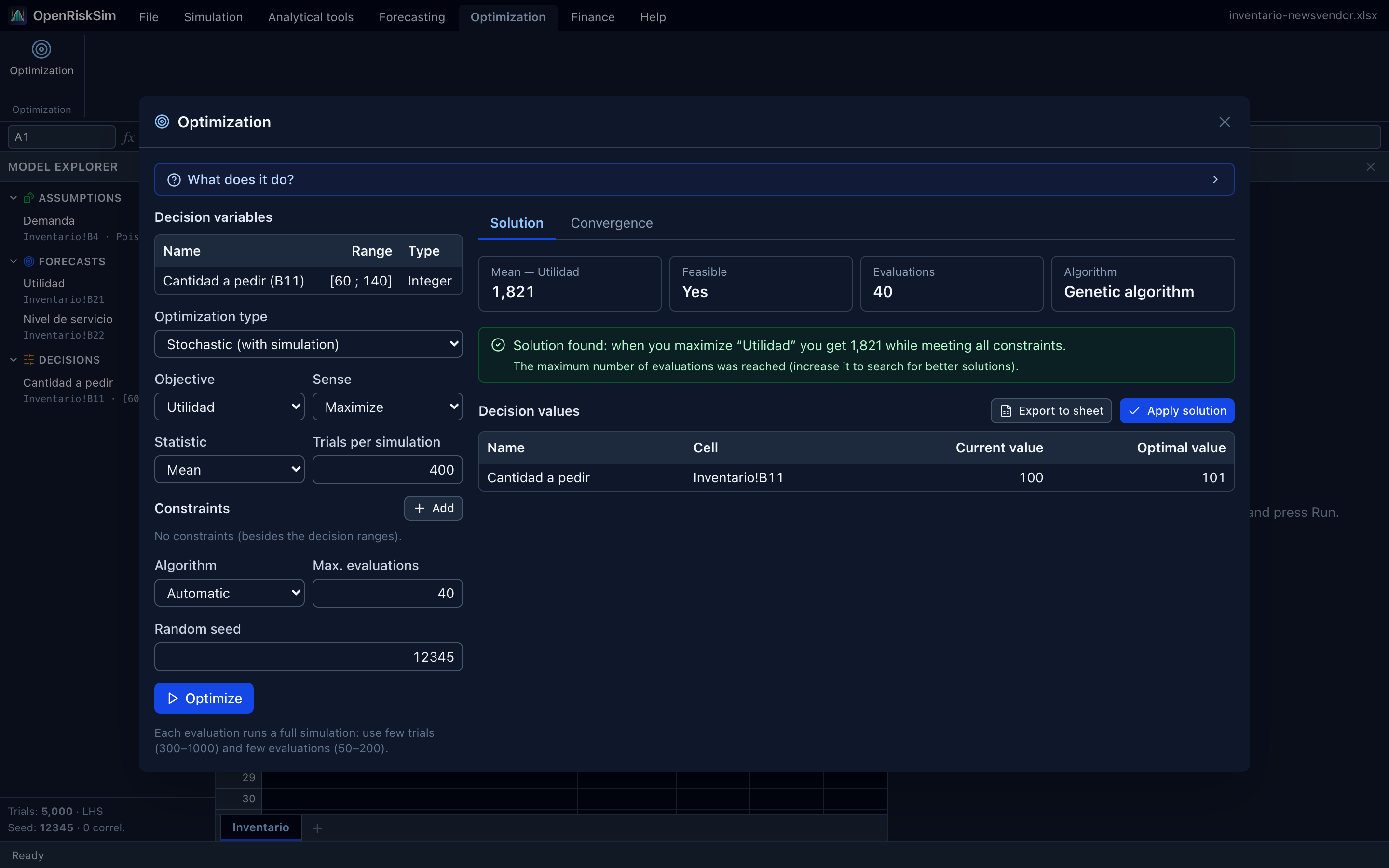
- Cards with the objective's best value, whether it is Feasible, the number of Evaluations and the Algorithm used.
- A message with the conclusion (“Solution found: when you maximize ‘Utilidad’ you get…”) and the reason it stopped (converged, evaluation budget reached, stopped by the user).
- Decision values: Current value and Optimal value of each.
- Status of each constraint (Condition, Value, Met?).
- Apply solution writes the optimal values into the decision cells. Export to sheet saves the table.
Convergence tab. Best value versus evaluations. If the curve is still rising at the end, increase Max. evaluations.
Efficient frontier tab. See below.
Always verify
Optimization algorithms don't guarantee the global optimum on hard problems. Try another seed or algorithm and, after Apply solution, run a regular simulation with more trials to confirm.
Efficient frontier
Tick Efficient frontier (vary a constraint's limit), choose the constraint and the range of limits (from, to, number of steps). The tool re-optimizes for each limit and plots the optima. Each point shows how much objective you gain by relaxing the constraint: e.g. more expected return for more risk.
Example with Investment portfolio: objective = maximize the mean Retorno de la cartera (portfolio return, stochastic), constraints Cartera!E10 = 1 (weights sum to 1) and forecast Retorno de la cartera with statistic Standard deviation <= limit. Varying the limit, e.g. from 4% to 14%, traces Markowitz's risk–return frontier.
Example: inventory (newsvendor)
Open File → Examples → Inventory (newsvendor). Demand is Poisson with mean 100; each unit costs $30 and sells for $50, leftovers are salvaged at $10 and each shortage costs $5 of goodwill. The decision is the order quantity (B11, integer between 60 and 140).
- Optimization → Optimization.
- Optimization type: Stochastic (with simulation).
- Objective: Utilidad (profit); Sense: Maximize; Statistic: Mean.
- Trials per simulation: 400; Max. evaluations: 40 (few combinations are possible); Algorithm: Automatic (will pick the genetic algorithm since the variable is integer).
- Optimize.
Result: the optimal quantity is ≈ 101 units, with mean profit around $1,820. This matches newsvendor theory: the optimal quantity is the demand quantile at the critical ratio (price − cost + penalty) / (price − salvage + penalty) = 25/45 ≈ 0.556 (computed in the example's cell B24), which for a Poisson(100) is ≈ 101.
Then try minimizing Prob. at or below threshold of profit with threshold 1,500, or add a constraint on the Nivel de servicio forecast (fill rate; statistic Mean, >= 0.95), and see how the decision changes.