
Finance
The Finance tab gathers the classic project-evaluation tools. None needs a simulation and almost all have Export to sheet.
Conventions: rates are typed as percentages in fields marked %; cash flows start at period 0 (usually the investment, negative), which is not discounted.
Project evaluator
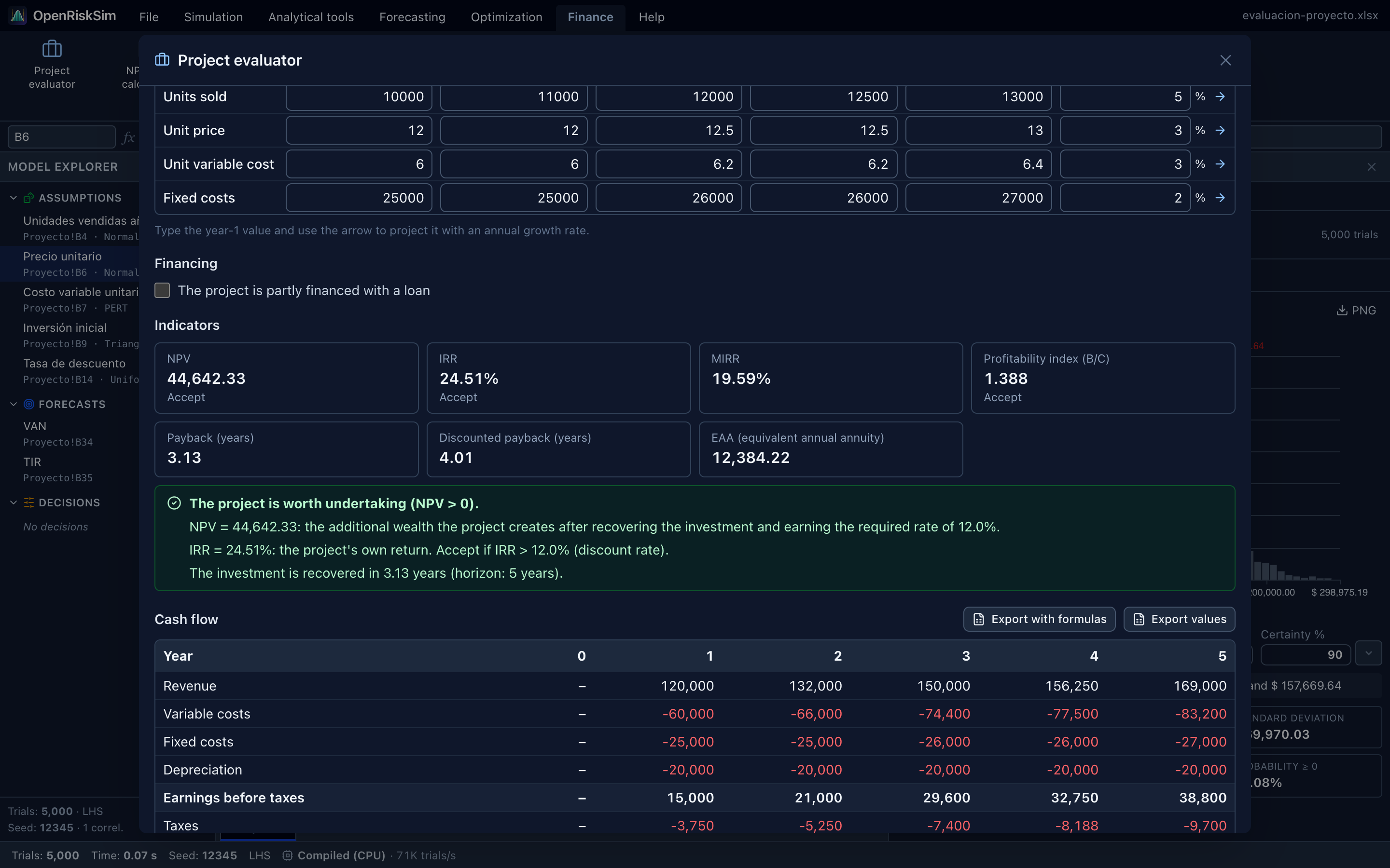
Purpose. Builds a project's full cash flow — revenue, costs, depreciation, taxes, investment, working capital and salvage value — and computes the profitability indicators. With financing, it also computes the equity cash flow. Export with formulas turns the cash flow into a live sheet ready for risk analysis.
How to use it.
- General data: Horizon (years), Initial investment (fixed assets), Working capital, Salvage value (sale value of the assets at the end), Depreciation method (straight line, double declining balance or sum of years' digits), Useful life (years), Tax rate and Discount rate (hurdle rate / WACC).
- Per-year data: Units sold, Unit price, Unit variable cost and Fixed costs for each year. Type year 1, set a Growth rate and click the → arrow to project the other years.
- Financing (optional): tick The project is partly financed with a loan and enter Loan amount, Loan rate, Term (years) and the amortization method.
Results update instantly.
How the cash flow is built
Project (free) cash flow:
Equity cash flow (with a loan):
Indicators
| Indicator | Formula | Rule |
|---|---|---|
| NPV | NPV = Σₜ CFₜ / (1 + i)ᵗ, t = 0…n | NPV > 0 ⇒ accept: the extra wealth after recovering the investment and earning the required rate i. |
| IRR | Rate r such that Σₜ CFₜ / (1 + r)ᵗ = 0 | IRR > i ⇒ accept. |
| MIRR | MIRR = (FV of positive flows at the reinvestment rate / |PV of negative flows at the finance rate|)^(1/n) − 1 | Fixes the reinvest-at-IRR assumption and is always unique. In the evaluator both rates equal the discount rate. |
| Profitability index (B/C) | PI = PV of flows t = 1…n / |CF₀| = 1 + NPV / |CF₀| | PI > 1 ⇒ accept. |
| Payback (years) | Period when the cumulative flow becomes ≥ 0, interpolated within the year | Lower is better; measures liquidity, not profitability. |
| Discounted payback (years) | Same, with discounted flows | Always ≥ payback. |
| EAA (equivalent annual annuity) | EAA = NPV × i / (1 − (1 + i)⁻ⁿ) | To compare projects of different lengths. |
| Equity NPV / IRR | Same calculations on the equity cash flow | Compare the equity IRR with the cost of equity (Ke). |
The evaluator shows a verdict (“The project is worth undertaking (NPV > 0)”), explains each indicator and warns when the cash flow changes sign several times and has more than one IRR: decide with NPV or MIRR then.
Below are the Cash flow table and the NPV profile (NPV versus discount rate: the IRR is where the curve crosses zero).
Export
- Export with formulas: creates a
Projectsheet (Proyectowith the Spanish interface) with a live model (formulas that exactly reproduce the evaluator's calculations). The message tells you the NPV cell and the price and units cells. From there: define a forecast on the NPV and assumptions on the data cells, and run the simulation. See the tutorial. - Export values: creates a
Project (values)sheet with plain numbers (for appendices or reports).
NPV/IRR calculator
Purpose. Computes every indicator for any cash flow: NPV, IRR (and all IRRs if the flow changes sign several times), MIRR, payback, discounted payback, profitability index and EAA.
How to use it. In Cash flows (period 0, 1, 2…) paste or select the flows (investments and outflows negative), and set the Discount rate, Finance rate (MIRR) and Reinvestment rate (MIRR). Click Calculate.
How to read it. Besides the indicators, it shows the Flows and cumulative chart (cash flow, cumulative and discounted cumulative: payback is where the cumulative crosses zero) and a table with each period's Discount factor and Present value. If the flow never changes sign, it warns that no IRR exists.
Multiple IRRs
A flow like −100, +230, −132 (investment, income, closing cost) has two IRRs: 10% and 20%. The calculator shows both. When there is more than one, the IRR is useless as a criterion: use NPV or MIRR.
Loan amortization
Purpose. Builds the amortization schedule and compares methods.
How to use it. Enter Loan amount, Rate per period (monthly if payments are monthly: 12% nominal annual ⇒ 1% monthly), Number of payments and Amortization method:
| Method | Payment | Behaviour |
|---|---|---|
| French (level payment) | P = L × i / (1 − (1 + i)⁻ⁿ) | All payments equal; mostly interest at first, principal at the end. |
| German (level principal) | Principal = L / n; payment = L/n + interest on the balance | Payments decrease over time. |
| American (bullet) | Interest only (L × i); full principal in the last payment | Lower initial burden, higher total interest. |
How to read it. You get First payment, Last payment, Total paid, Total interest, a comparison of total interest across the three methods, the Payment breakdown and Outstanding balance charts, and the Amortization schedule (Payment, Interest, Principal, Balance).
Depreciation
Purpose. Compares depreciation methods for an asset: Straight line, Declining balance, Double declining balance, Sum of years' digits and Units of production (for the latter, enter the Units produced per year).
How to use it. Enter Asset cost, Salvage value and Useful life (years).
How to read it. Every method depreciates the same total (cost − salvage); only the timing changes. Accelerated methods depreciate more early on: since depreciation reduces taxes, they bring the tax saving forward and increase the NPV. The Annual depreciation and Book value for each method are shown as chart and table.
| Method | Depreciation in year t |
|---|---|
| Straight line | (C − S) / n |
| Sum of years' digits | (C − S) × (n − t + 1) / [n(n + 1)/2] |
| Declining balance | fixed rate 1 − (S/C)^(1/n) × book value (like Excel DB) |
| Double declining balance | 2/n × opening book value, switching to straight line when larger and never below salvage (like Excel DDB/VDB) |
| Units of production | (C − S) × year's units / total units |
Cost of capital
Purpose. Computes the project's discount rate. Three tabs:
CAPM. Cost of equity with country risk:
Fields: Risk-free rate, Market return, Country risk (EMBI spread) and Beta. Optionally, Compute the levered beta from the industry's unlevered beta (Hamada):
with Unlevered beta, Debt / Equity and Tax rate. Useful in emerging markets: take the industry beta from developed markets (e.g. Damodaran's tables), relever it with your capital structure and add country risk.
WACC. Weighted average cost of capital:
Fields: Equity (E), Debt (D), Tax rate, Cost of equity (Ke) (or Use the CAPM cost of equity) and Cost of debt (Kd). WACC discounts the project cash flow; Ke, the equity cash flow.
Rate conversion.
- Nominal → effective: EAR = (1 + j/m)ᵐ − 1, with m = Compounding periods per year (12 monthly, 4 quarterly, 2 semi-annual).
- Effective → nominal / periodic: periodic rate = (1 + EAR)^(1/m) − 1; nominal = periodic × m.
- Real rate (Fisher): (1 + nominal) = (1 + real) × (1 + inflation). Use the real rate for constant-currency flows and the nominal rate for flows that include inflation.
Break-even
Two tabs:
Accounting. Quantity to sell for zero profit:
With Expected sales (units) it also computes the Margin of safety (how much sales can fall before losses). Shows the Revenue vs Total cost chart. If the price doesn't exceed the variable cost there is no break-even point.
NPV = 0 (model). Searches for the value of a workbook input cell (price, units, cost…) that makes a forecast (such as the NPV) equal a Target value (0 by default), searching between Search from and Search to. Answers: how much can this variable worsen before the project stops being worthwhile? You get the Critical value, Current value, Required change (%) and the forecast curve versus the cell.
Use it with the simulation
If the critical price is $22.30 and the current price $26, the price can fall ≈ 14% before the NPV turns negative. Compare that with the distribution you gave the price: how likely is it to fall below?
Scenario analysis
Purpose. The simplified version of risk analysis: combine scenarios (Pessimistic, Base, Optimistic and any you add with Add scenario) with their Probabilities and a Value (e.g. each scenario's NPV).
How to read it. Computes the Expected value E = Σ pᵢ·NPVᵢ, the Standard deviation σ = √Σ pᵢ·(NPVᵢ − E)², the Coefficient of variation σ/|E| (CV > 1 ⇒ high risk relative to the expected value) and the Probability of a negative value (sum of probabilities of scenarios with value < 0). Probabilities not summing to 100% are normalised.
Monte Carlo simulation generalises this idea to thousands of scenarios: for a complete analysis, define assumptions on the key variables and run a simulation.