
Quick start (5 minutes)
In this walkthrough you will open the “Project evaluation” example, see how its risk model is built, run the simulation and read the probability that the NPV is positive.
1. Open the example
- Open the app.
- In the ribbon, File tab, click Examples.
- Choose Project evaluation. If a workbook was already open, the app asks you to confirm that it will be replaced (and that autosave will be overwritten).
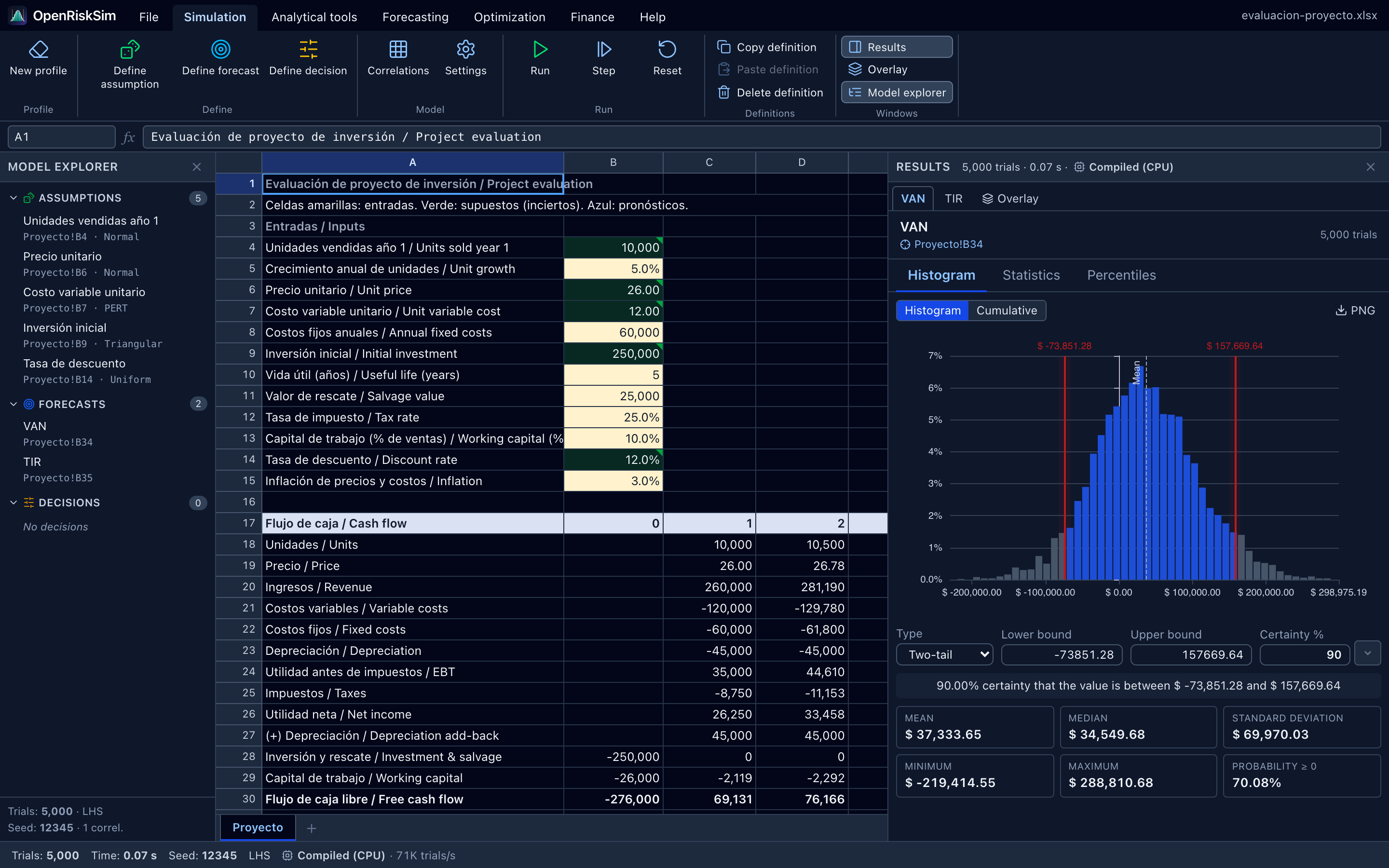
The Proyecto sheet appears: inputs at the top (rows 4–15), the 5-year cash flow in the middle (rows 17–31) and the indicators (NPV, IRR, payback…, rows 34–38) at the bottom. Labels are bilingual.
2. Look at the assumptions (green cells)
Cells shaded green are assumptions: uncertain variables with a probability distribution. The Model explorer panel (left) lists them all:
| Assumption | Cell | Distribution |
|---|---|---|
| Units sold year 1 | B4 | Normal (mean 10,000, sd 1,500), truncated at minimum 0 |
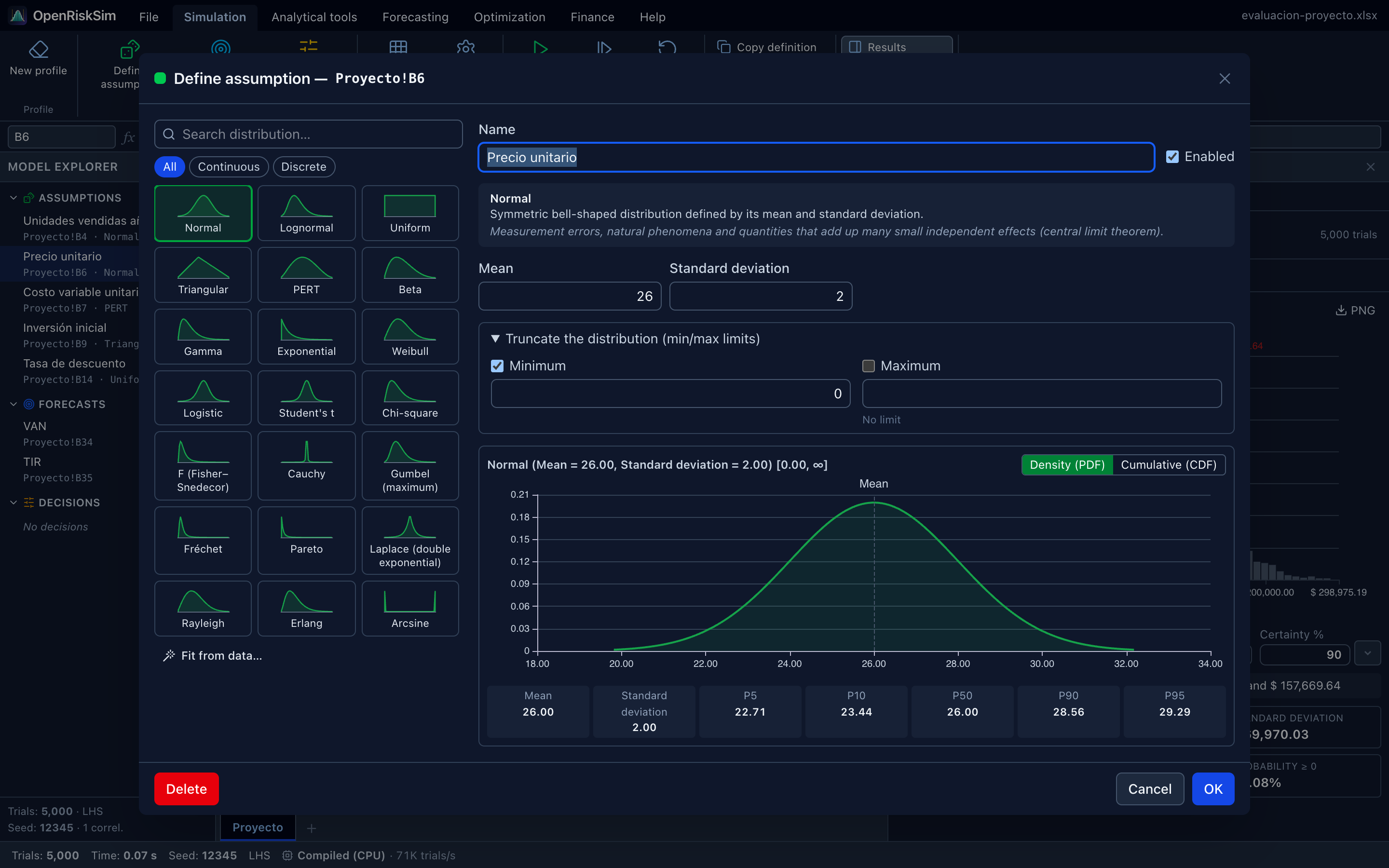
| Unit price | B6 | Normal (mean 26, sd 2), truncated at minimum 0 |
| Unit variable cost | B7 | PERT (min 10.5, most likely 12, max 15) |
| Initial investment | B9 | Triangular (min 220,000, most likely 250,000, max 310,000) |
| Discount rate | B14 | Uniform (0.10 to 0.14) |
There is also a −0.5 correlation between price and units: when the price goes up, sales tend to go down. (Assumption names in the example are in Spanish, e.g. “Precio unitario”.)
Select cell B6 and click Simulation → Define assumption (or right-click the cell, or Alt+A) to see its definition: the distribution gallery, parameters, truncation and the distribution chart. Click Cancel to leave without changes.
3. Look at the forecasts (blue cells)
Blue cells are forecasts: the results recorded in each trial. In this example they are the NPV (B34, named “VAN”) and the IRR (B35, named “TIR”). Both are formulas that depend, directly or indirectly, on the green cells.
4. Run the simulation
Click Simulation → Run (or Alt+R). The example is set to 5,000 trials, Latin hypercube sampling and fixed seed 12345, so in under a second the Results panel opens on the right.
Same numbers as your classmate
With a fixed seed, anyone running the example with the same settings gets exactly the same results. Handy for group work and exams.
5. Read the histogram and the certainty
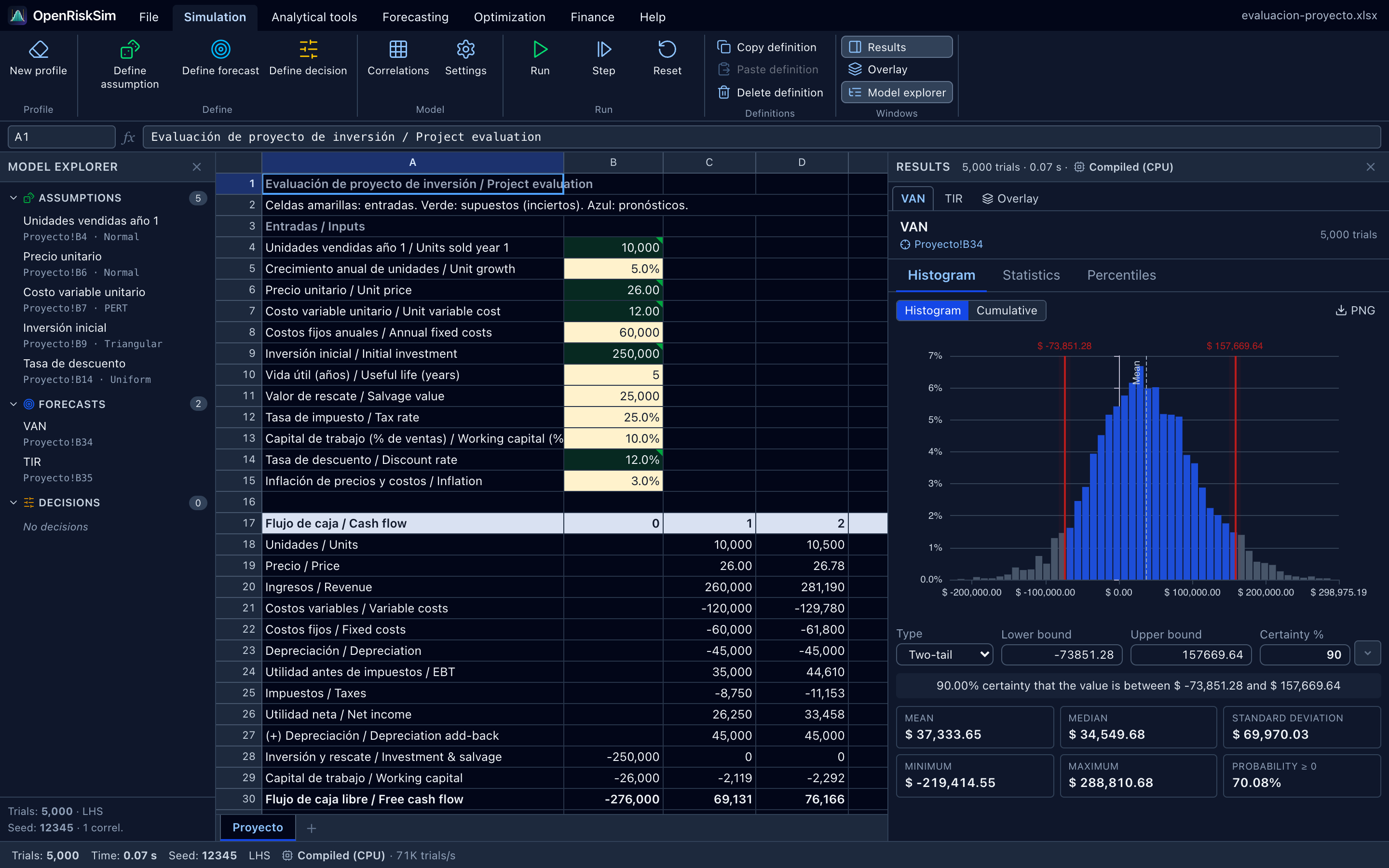
In the NPV tab of the results panel you'll see:
- The histogram of the 5,000 simulated NPVs. Central bars (blue) are inside the certainty interval; grey ones are outside.
- Below, the certainty controls: by default Two-tail with Certainty % = 90, i.e. the interval that leaves 5% of trials on each side. The sentence below summarises it: “90.00% certainty that the value is between $ −73,851.28 and $ 157,669.64”.
- Cards with Mean (≈ $37,334), Median, Standard deviation, Minimum, Maximum and Probability ≥ 0 (≈ 70%).
Now answer the key question — what is the probability that the project is profitable?:
- In Type, choose Right-tail ≥.
- In Lower bound, type
0. - Certainty % is recomputed: ≈ 70%. There is a 70% probability that the NPV is greater than or equal to zero and therefore a 30% probability of loss.
You can also drag the red vertical lines on the histogram with the mouse to move the bounds.
6. What next?
- Click Analytical tools → Tornado to see which variables move the NPV the most.
- Change the number of trials in Simulation → Settings and run again.
- Export the report with File → Export report.
- Do the full tutorial, which builds and analyses this model like a course assignment.
- Learn to define your own assumptions on your file.