Analytical tools
The Analytical tools tab gathers nine tools to understand what drives risk, describe data and choose distributions. Each opens in its own window, has a What does it do? box with a short explanation and, in most cases, an Export to sheet button that copies the result table to a new sheet.
| Tool | Requires a simulation? | Question it answers |
|---|---|---|
| Tornado | No | Which variables move the result most, one at a time? |
| Spider chart | No | How does the result respond to each variable across its range? |
| Sensitivity | Yes | Which assumptions explain the forecast's variance in the simulation? |
| Scenario table | No | What is the result for combinations of two variables? |
| Distribution fitting | No | Which distribution best describes my data? |
| Bootstrap | Optional | How precise is a statistic? |
| Hypothesis test | Optional | Are the means of two samples different? |
| Descriptive statistics | Optional | What do my data look like? |
| Overlay chart | Yes | How do several forecasts compare? |
Data sources
Tools that work with data (fitting, bootstrap, hypothesis test, descriptive statistics) offer up to three sources:
- Sheet range: type a range such as
Sheet1!B2:B40, click Use selection to take the selected range, or the pick button to select it on the sheet (the dialog hides while you select). - Paste data: paste numbers separated by new lines, tabs or
;. - Simulated forecast: the values of a forecast from the last simulation.
Tornado
Purpose. The classic “one variable at a time” sensitivity analysis. It moves each assumption from a low percentile to a high percentile of its distribution (P10 and P90 by default) while keeping the others at their base value (the cell's current value), and measures how much the forecast changes.
How to use it.
- Choose the Forecast.
- Choose the Method:
- Distribution percentiles (default): adjust Low percentile (%) and High percentile (%) if you like (e.g. 5 and 95 for wider ranges).
- ± % of base value (like Risk Simulator): moves every variable by the same percentage (Change ±, 10 % by default), regardless of its distribution.
- If several assumptions share the same name (e.g. "Production" in years 1, 2 and 3), tick Group assumptions with the same name to move them together as one variable. They show up as "Production (×3)".
- Click Calculate.
How to read it.
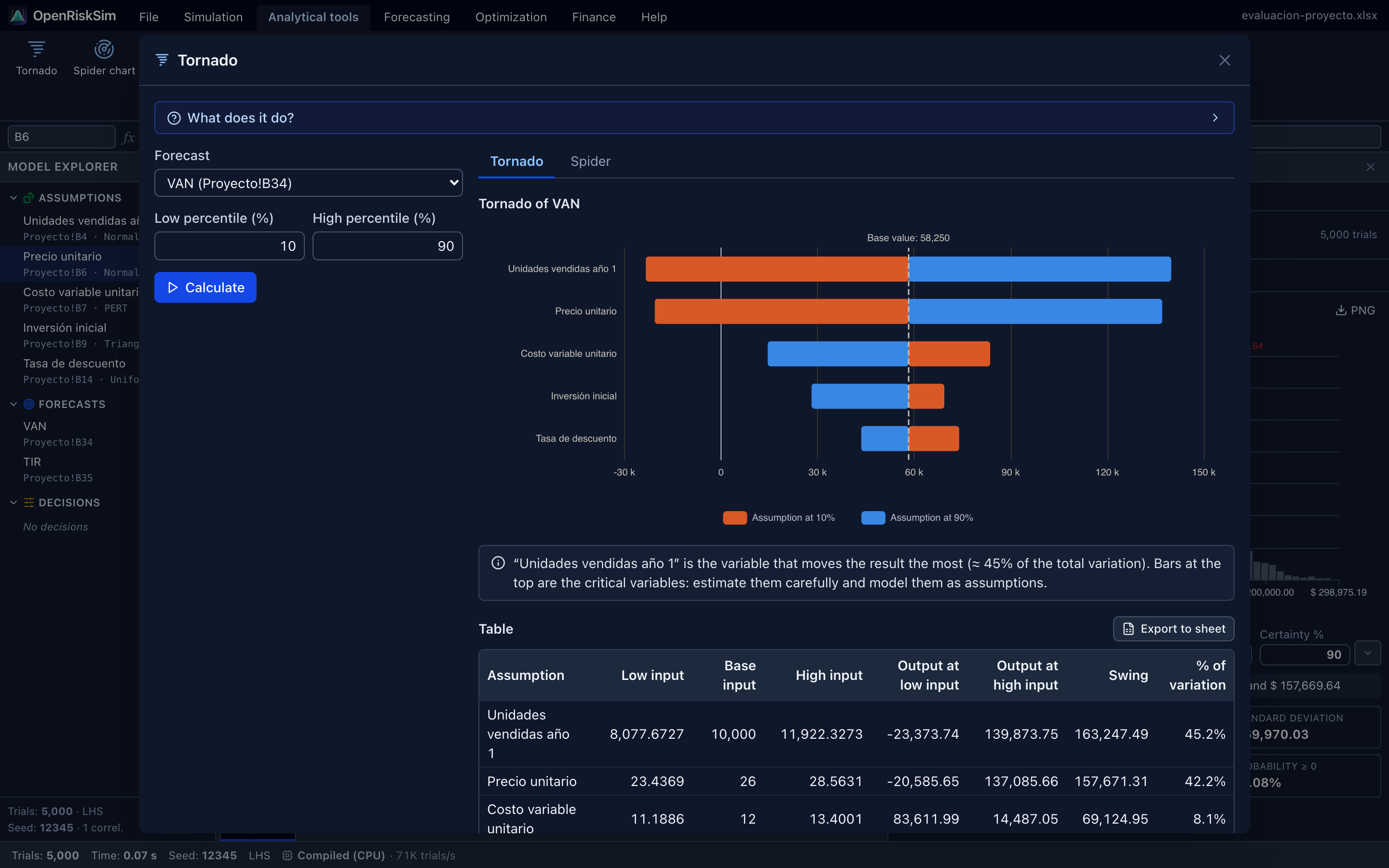
- Bars are sorted by swing (difference between the result at the low and at the high input). The top ones are the critical variables: estimate them more carefully.
- Colours: orange = assumption at the low percentile, blue = at the high percentile. Blue on the right means a direct relationship (variable up, result up); blue on the left, an inverse one.
- The table shows Low input, Base input, High input, Output at low / high input, Swing and % of variation (squared swing over the sum of squared swings).
- A bar crossing the NPV's zero line means that variable alone can make the project unprofitable.
TIP
The tornado doesn't need a simulation and is fast. Use it at the start to decide which variables to model as assumptions, and at the end to explain the risk in your report.
Why doesn't my tornado have the same order as Risk Simulator's?
By default Risk Simulator moves each variable ±10 % of its base value. With percentiles, OpenRiskSim uses the uncertainty you defined: a variable with a wide or skewed distribution (e.g. variable costs triangular 3.5 – 4 – 6, whose P90 is 32 % above base) weighs more than one with little room (production 16,000 – 20,000 – 20,500, whose P90 is only 0.1 % above). Both are right but answer different questions:
- ± %: which variable moves the result most if they all change by the same amount?
- Percentiles: which variable moves the result most given each one's real uncertainty?
Also, if one concept is spread over several cells with separate assumptions, group them so the tornado doesn't split its effect into several small bars. To reproduce Risk Simulator use ± % of base value at 10 % and group.
Limitation
By moving one variable at a time, the tornado ignores correlations and interactions. For the contribution to risk “with everything varying together”, use Sensitivity.
Spider chart
Purpose. Complements the tornado: instead of two points it sweeps several percentiles of each assumption (9 Spider points by default) and draws one line per variable.
How to use it. Choose the forecast and the number of points, and click Calculate. It is also available as the Spider tab inside the tornado window.
How to read it. The horizontal axis is the assumption percentile; the vertical one, the forecast. The steeper the line, the more sensitive the result to that variable; a flat line means it barely matters. Curvature reveals non-linear effects (e.g. taxes paid only on profits). The chart shows the most influential variables; the table includes all.
Sensitivity
Purpose. Uses the last simulation to measure the relationship between each assumption and the forecast with every variable moving together (correlations included).
How to use it. Run the simulation, open Sensitivity and choose the forecast.
How to read it.
- Rank correlation (Spearman, −1 to 1): direction and strength. Positive: when the assumption rises, the forecast rises; negative: it falls.
- Contribution to variance: what share of the forecast's uncertainty each assumption explains (squared correlation normalised to sum to 100%). This is what Risk Simulator shows in its sensitivity chart.
- Correlations near 0 (|ρ| < 0.1) mean little influence: you can fix those variables at their base value to simplify the model.
Scenario table
Purpose. Computes the forecast for every combination of two assumptions, like an Excel two-variable “data table”. Other assumptions stay at their base value.
How to use it.
- Choose the Forecast.
- Choose the Assumption in rows and the Assumption in columns (must differ), with their From/To range (P10 to P90 of each distribution is suggested) and number of Steps.
- Click Calculate.
How to read it. Red cells are combinations with a negative result (e.g. NPV < 0 ⇒ project not worth it); blue, positive. It shows the profitability “frontier”: e.g. the minimum price needed for each sales level.
Distribution fitting
Purpose. Finds the probability distribution that best describes historical data, to use as an assumption. Equivalent to Risk Simulator's Distributional Fitting.
How to use it.
- Choose the Data (range, paste or simulated forecast). The more data the better: with fewer than 30 points the results are indicative.
- Rank by: AIC (default), BIC, Kolmogorov–Smirnov or Anderson–Darling.
- Data type: Automatic (if all values are integers, discrete distributions are tried), Continuous or Discrete (integers).
- Click Fit. 24 continuous distributions (Normal, Lognormal, Gamma, Weibull, Beta, Triangular, PERT…) or 6 discrete ones (Poisson, Binomial, Negative binomial, Geometric, Bernoulli, Discrete uniform) are fitted by maximum likelihood. Those that can't fit the data (e.g. a Lognormal with negative data) are skipped.
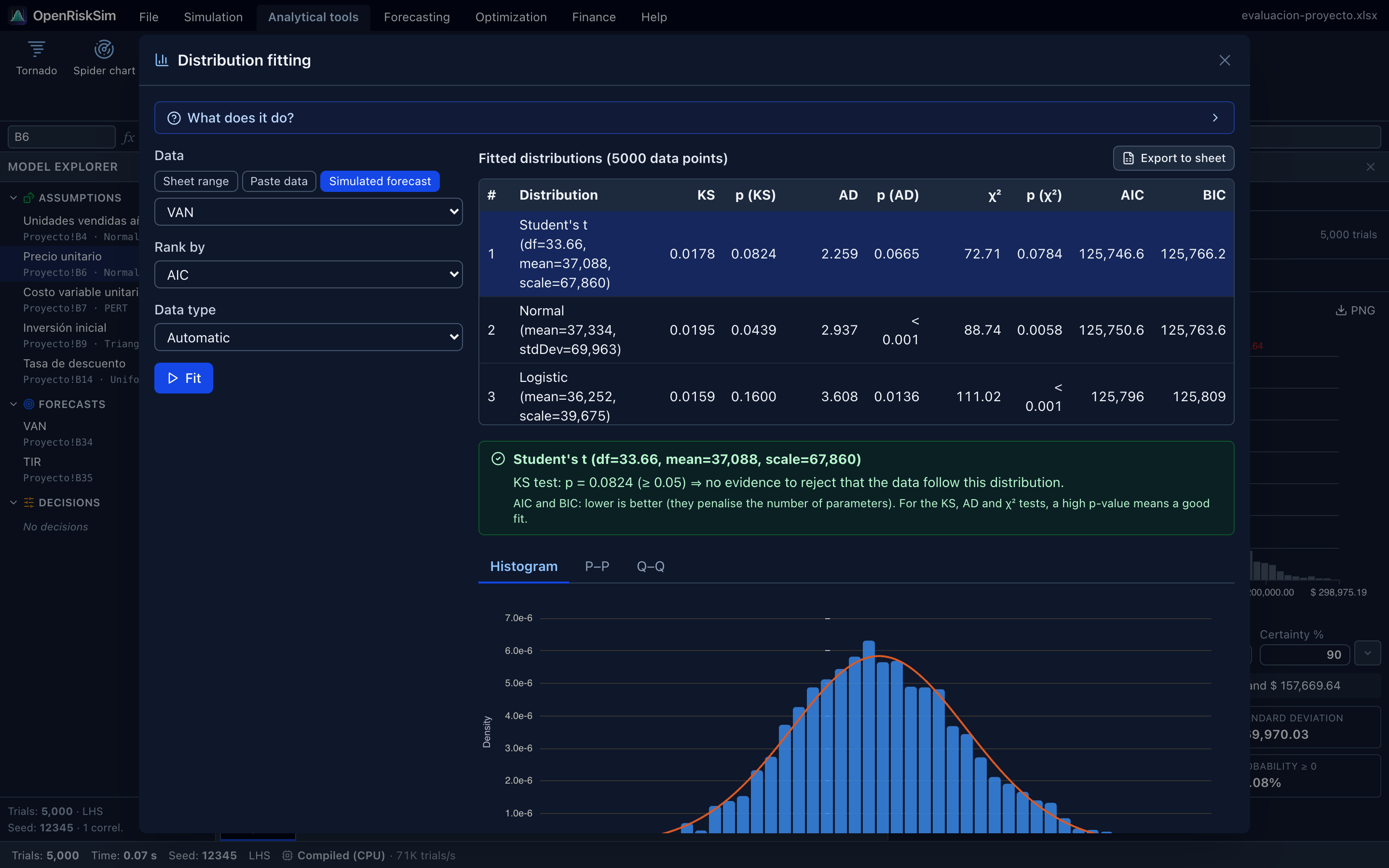
- The Fitted distributions table shows each candidate's estimated parameters, the KS, AD and χ² statistics with their p-values, and AIC and BIC. Below, a box summarises whether the KS test rejects the selected distribution.
- Select a row to see the Histogram with the fitted curve and the P–P and Q–Q plots.
- Under Use in the model, select a cell on the sheet and click Create assumption with this distribution. If the cell already has an assumption, its distribution is replaced.
How to read the criteria.
| Criterion | Rule | Comment |
|---|---|---|
| AIC / BIC | Lower is better | Reward fit (likelihood) and penalise the number of parameters. BIC penalises more, so it prefers simpler models. Only for comparing distributions on the same data. |
| p (KS) | Higher is better; p ≥ 0.05 ⇒ fit not rejected | Kolmogorov–Smirnov: largest distance between empirical and theoretical CDFs. Sensitive to the centre. |
| p (AD) | Higher is better | Anderson–Darling: like KS but weighting the tails more. Continuous only. |
| p (χ²) | Higher is better | Chi-square goodness of fit with equiprobable bins (or one bin per integer for discrete data). |
P–P and Q–Q plots. If the points follow the diagonal, the distribution describes the data well. P–P is more sensitive to the centre; Q–Q to the tails (extreme values).
p-values are approximate
Because parameters are estimated from the same data being tested, KS and AD p-values are conservative (tend to be higher than they should), except AD for Normal and Lognormal, which uses the D'Agostino–Stephens correction. Use them to rank candidates and discard clearly bad ones, not as a formal test. And always choose a distribution that makes sense for the variable.
None fits well?
If every p is below 0.05, consider using the data directly through the Custom (empirical) distribution. See Assumptions → Custom distribution.
Bootstrap
Purpose. Estimates how precise a statistic (mean, median, standard deviation, percentile…) is without assuming any distribution, by resampling the data with replacement many times and computing the statistic on each resample.
How to use it. Choose the Data (a simulated forecast by default), the Statistic (Mean, Median, Standard deviation, Coefficient of variation, 5th/10th/90th/95th percentile, Skewness or Kurtosis), the number of Resamples (2,000 by default), the Confidence and the Random seed, and click Calculate.
How to read it. You get the Estimate, the confidence interval (percentile method), the Standard error (bootstrap) and a histogram of the bootstrap distribution. Example: “With 95% confidence, the true 5th percentile of the NPV is between X and Y”. A very wide interval means an imprecise statistic: add simulation trials.
Hypothesis test
Purpose. Compares the means of two samples: two simulated forecasts (the NPV of alternative A and of B) or two data ranges, with Welch's t-test, which doesn't assume equal variances.
How to use it. Choose Sample A and Sample B, the Significance α (0.05 by default) and the Alternative hypothesis (Mean A ≠ mean B, Mean A > mean B or Mean A < mean B), and click Test.
How to read it. H₀: the means are equal. If the p-value is below α, H₀ is rejected and the difference is statistically significant. You also get the t statistic, Degrees of freedom, the CI of the difference (A − B), a summary of each sample and their cumulative distributions.
Significant is not the same as important
With thousands of simulated trials, even tiny differences become “significant”. Also look at the size of the difference and its confidence interval.
Descriptive statistics
Purpose. Summarises a data set: count, mean, median, mode (approx.), standard deviation, variance, coefficient of variation, minimum, maximum, range, skewness, kurtosis (excess), standard error and 95% CI of the mean, plus a percentile table. Draws the Histogram and Cumulative distribution.
How to read it. The tool writes an automatic interpretation: where the data are centred, whether there is skew (mean above median ⇒ tail towards high values) and whether tails are heavier than a Normal's. A good first step before distribution fitting.
Overlay chart
Purpose. Overlays the simulated distributions of several forecasts (up to 8) to compare them, e.g. the NPV of two investment alternatives.
How to use it. Tick the Forecasts, choose Frequencies (PDF) or Cumulative (CDF) and the Number of bins (40 by default). A Summary with each one's statistics appears below.
How to read it. A curve shifted to the right has higher values; a wider one, more risk. In the cumulative view, if A's curve is always below and to the right of B's, A is better at every probability level (stochastic dominance).